Colpitts oscillator

Jump to: navigation, search

Early schematic of a Colpitts circuit, using a vacuum tube, redrawn from the patent publication.

A Colpitts oscillator, invented in 1920 by American engineer Edwin H. Colpitts, is one of a number of designs for electronic oscillator circuits using the combination of an inductance (L) with a capacitor (C) for frequency determination, thus also called LC oscillator. The distinguishing feature of the Colpitts circuit is that the feedback signal is taken from a voltage divider made by two capacitors in series. One of the advantages of this circuit is its simplicity; it needs only a single inductor. Colpitts obtained US Patent 1624537^[1] for this circuit.
The frequency is generally determined by the inductor and the two capacitors at the bottom of the drawing.

Implementation

Figure 1: Simple common base Colpitts oscillator (with simplified biasing)	Figure 2: Simple common collector Colpitts oscillator (with simplified biasing)
Figure 3: Practical common base Colpitts oscillator (with an oscillation frequency of ~50 MHz)

A Colpitts oscillator is the electrical dual of a Hartley oscillator. Fig. 1 shows the basic Colpitts circuit, where two capacitors and one inductor determine the frequency of oscillation. The feedback needed for oscillation is taken from a voltage divider made of two capacitors, whereas in the Hartley oscillator the feedback is taken from a voltage divider made of two inductors (or a single, tapped inductor).
As with any oscillator, the amplification of the active component should be marginally larger than the attenuation of the capacitive voltage divider, to obtain stable operation. Thus, a Colpitts oscillator used as a variable frequency oscillator (VFO) performs best when a variable inductance is used for tuning, as opposed to tuning one of the two capacitors. If tuning by variable capacitor is needed, it should be done via a third capacitor connected in parallel to the inductor (or in series as in the Clapp oscillator).
Fig. 2 shows an often preferred variant, where the inductor is also grounded (which makes circuit layout easier for higher frequencies). Note that feedback energy is fed into the connection between the two capacitors. This amplifier provides current, not voltage, amplification.
Fig. 3 shows a working example with component values. Instead of bipolar junction transistors, other active components such as field effect transistors or vacuum tubes, capable of producing gain at the desired frequency, could be used.

Theory

Oscillation frequency

The ideal frequency of oscillation for the circuits in Figures 1 and 2 are given by the equation: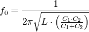

$f_0 = {1 \over 2 \pi \sqrt {L \cdot \left ({ C_1 \cdot C_2 \over C_1 + C_2 }\right ) }}$

where the series combination of C1 and C2 creates the effective capacitance of the LC tank.
Real circuits will oscillate at a slightly lower frequency due to junction capacitances of the transistor and possibly other stray capacitances.

Instability criteria

This section may require cleanup to meet Wikipedia's quality standards. (Consider using more specific cleanup instructions.) Please help improve this section if you can. The talk page may contain suggestions. (April 2008)

Colpitts oscillator model used in analysis at left.

One method of oscillator analysis is to determine the input impedance of an input port neglecting any reactive components. If the impedance yields a negative resistance term, oscillation is possible. This method will be used here to determine conditions of oscillation and the frequency of oscillation.
An ideal model is shown to the right. This configuration models the common collector circuit in the section above. For initial analysis, parasitic elements and device non-linearities will be ignored. These terms can be included later in a more rigorous analysis. Even with these approximations, acceptable comparison with experimental results is possible.
Ignoring the inductor, the input impedance can be written as

$Z_{in} = \frac{v_1}{i_1}$

Where $v_1$ is the input voltage and $i_1$ is the input current. The voltage $v_2$ is given by

$v_2 = i_2 Z_2$

Where $Z_2$ is the impedance of $C_2$ . The current flowing into $C_2$ is $i_2$ , which is the sum of two currents:

$i_2 = i_1 + i_s$

Where $i_s$ is the current supplied by the transistor. $i_s$ is a dependent current source given by

$i_s = g_m \left ( v_1 - v_2 \right )$

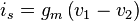
Where $g_m$ is the transconductance of the transistor. The input current $i_1$ is given by

$i_1 = \frac{v_1 - v_2}{Z_1}$

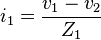
Where $Z_1$ is the impedance of $C_1$ . Solving for $v_2$ and substituting above yields

$Z_{in} = Z_1 + Z_2 + g_m Z_1 Z_2$

The input impedance appears as the two capacitors in series with an interesting term, $R_{in}$ which is proportional to the product of the two impedances:

$R_{in} = g_m \cdot Z_1 \cdot Z_2$

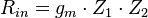If $Z_1$ and $Z_2$ are complex and of the same sign, $R_{in}$ will be a negative resistance. If the impedances for $Z_1$ and $Z_2$ are substituted, $R_{in}$ is

$R_{in} = \frac{-g_m}{\omega ^ 2 C_1 C_2}$

If an inductor is connected to the input, the circuit will oscillate if the magnitude of the negative resistance is greater than the resistance of the inductor and any stray elements. The frequency of oscillation is as given in the previous section.
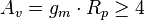
For the example oscillator above, the emitter current is roughly 1 mA. The transconductance is roughly 40 mS. Given all other values, the input resistance is roughly

$R_{in} = -30 \ \Omega$

This value should be sufficient to overcome any positive resistance in the circuit. By inspection, oscillation is more likely for larger values of transconductance and smaller values of capacitance. A more complicated analysis of the common-base oscillator reveals that a low frequency amplifier voltage gain must be at least four to achieve oscillation.^[2] The low frequency gain is given by:

$A_v = g_m \cdot R_p \ge 4$

If the two capacitors are replaced by inductors and magnetic coupling is ignored, the circuit becomes a Hartley oscillator. In that case, the input impedance is the sum of the two inductors and a negative resistance given by:

$R_{in} = -g_m \omega ^ 2 L_1 L_2$

In the Hartley circuit, oscillation is more likely for larger values of transconductance and larger values of inductance.

Oscillation amplitude

The amplitude of oscillation is generally difficult to predict, but it can often be accurately estimated using the describing function method.

STUDY MATERIAL for EC

Wednesday 9 May 2012

Colpitts oscillator

Contents

Implementation

Theory

Oscillation frequency

Instability criteria

Oscillation amplitude

No comments:

Post a Comment